
생각하는 감쟈
[Python] 5-2) 딥러닝 흐름2 본문

5DAY
기본 흐름 파악하기
선형모델
신경망 모델
출처 입력
기본 모델
가중치 / 입력 이미지 / 편향 / 스코어
선형 층
Dense(output, activation, input_shape)
output : 출력값의 개수
input_shape : 입력 벡터 형태
activation : 해당되는 경우에만 설정
손실함수 설정
|
문제종류
|
label 차원
|
activation
|
Loss이진 함수
|
|
이진분류
|
1 (0또는1)
|
sigmoid
|
binary_crossentropy
|
|
다중분류
|
n (One-hot 백터)
|
softmax
|
categorical_crossentropy
|
|
다중분류
|
n (숫자 0,1,2,...)
|
softmax
|
sparse_categorical_crossentropy
|
|
회귀
|
1 (실수)
|
-
|
mse / mae
|
compile
compile : loss, optimizer, metrics
loss : 손시 함수 설정 - loss='sparse_caegorical_crossentropy'
optimizer : 최적화 함수 설정 - optimzer='sgd'
metrice : 출력할 겂 설정 - metrice='acc'
학습설정
md.compile(loss='sparse_categorical_crossentropy', optimzer='sgd',metrics='acc')

hist = md.fit(train_x, train_y, epochs=200)
# 학습진행 상황을 hist에 저장
Danse()
Danse(n,activation=None)n = 출력츨 개수 설정
activation = 활성화 함수 설정
Danse = (3, activation='softmax', input_shape=(4,))#imput_shape : input data shape 설정(첫번째 층인 경우에 설정)
Sequential()
md = Sequential()
md.add(...)
-add(...) : 층을 추가
선형분류 coding 학습
from sklearn.datasets import load_iris
X, y = load_iris(return_X_y = True)

from sklearn.model_selection import train_test_split
train_x, test_x, train_y, test_y = train_test_split(X, y, test_size=0.3, random_state=42, stratify=y)
from tensorflow.keras.models import Sequential
from tensorflow.keras.layers import Dense
md = Sequential()
md.add(Dense(3, activation='softmax', input_shape=(4,)))
md.summary()md.compile(loss='sparse_categorical_crossentropy',
optimizer='sgd', metrics='acc')hist=md.fit(train_x, train_y, epochs=300, validation_split=0.2)loss = hist.history['loss']
val_loss = hist.history['val_loss']
epoch=np.arange(1, len(loss)+1)import matplotlib.pyplot as plt
plt.figure(figsize=(10,6))
plt.xlim(5, len(loss)+1)
plt.plot(epoch, loss, 'b', label='training loss')
plt.plot(epoch, val_loss, 'r', label='validation loss')
plt.legend()md.evaluate(test_x, test_y)
result = md.make_predict_function(test_x)
선형모델
이미지 데이터 : Gray image / Color Image
- 가장 작은 화소 단위인 픽셀 단위로 숫자화되어 저장
벡터화
- 선형 모델에서 입력 데이터는 벡터 형태로 처리된다
- 벡터화는 2차원 3차원 데이터를 1차원으로 변환하는 것
- 행렬과 벡터의 곱셈으로 처리되기에 입력 데이터가반드시 1차원 벡터 야만함
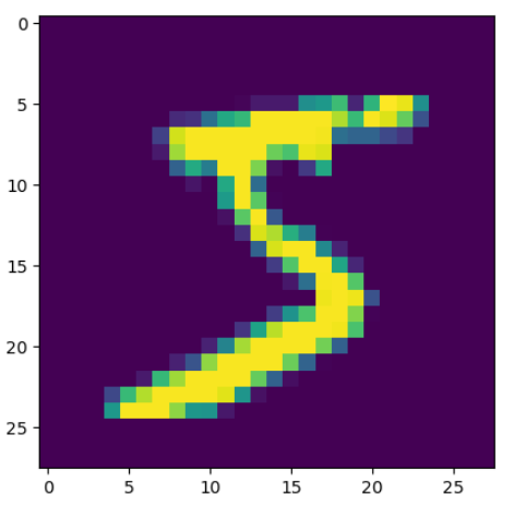
신경망모델 : Mnist
import numpy as np
import pandas as pd
from tensorflow.keras.datasets.mnist import load_data
(train_x, train_y), (test_x, test_y) = load_data()
train_x.shape, train_y.shape
test_x.shape, test_y.shape
from PIL import Image
img = train_x[0]

import matplotlib.pyplot as plt
img1 = Image.fromarray(img,mode='L')
plt.imshow(img1)
train_y[0]
train_x1 = train_x.reshape(60000,-1)
test_x1 = test_x.reshape(10000,-1)

train_x1.shape
test_x1.shape
train_x2 = train_x1/255
test_x2 = test_x1/255
from tensorflow.keras.models import Sequential
from tensorflow.keras.layers import Dense
md = Sequential()
md.add(Dense(10, activation='softmax', input_shape=(28*28,)))
md.summary()

md.compile(loss='sparse_categorical_crossentropy',optimizer='sgd', metrics='acc')
hist=md.fit(train_x2, train_y, epochs=30, batch_size=64, validation_split=0.2)
acc =hist.history['acc']
val_acc=hist.history['val_acc']
epoch=np.arange(1, len(acc)+1)
plt.figure(figsize=(10,8))
#plt.xlim(250, len(acc)+1)
plt.plot(epoch,acc,'b',label='acc')
plt.plot(epoch,val_acc, 'g', label='val_acc')
plt.legend()
md.evaluate(test_x2, test_y)
weight = md.get_weights()
weight
#plt.ylim(0.92, 0.94)
plt.plot(hist.history['loss'])
plt.plot(hist.history['val_loss'])
plt.title('model loss')
plt.ylabel('loss')
plt.xlabel('epoch')
plt.legend(['train', 'test'], loc='upper right')
plt.show()

#python #Ai #Bigdata #cloud #대외활동 #대학생 #daily
'Language > Python' 카테고리의 다른 글
| [Python] 기초_01 (0) | 2024.06.25 |
|---|---|
| [Python] 5-1) 딥러닝 흐름 (0) | 2023.06.10 |
| [Python] 4-4) 머신러닝 - 그래디언트,커널 (1) | 2023.06.10 |
| [Python] 4-3) 머신러닝 - 결정트리.. (1) | 2023.04.13 |
| [Python] 4-2) 머신러닝 - 지도학습 알고리즘 (1) | 2023.04.13 |
'Language/Python' Related Articles
more

Comments